Asset-Liability Matching (ALM)

The financial planning community has only recently begun attempting to incorporate portfolio spending goals into the portfolio construction process.  However, there is a lot of confusion over how to do this properly.  Many rely on Monte Carlo simulations and the ability to change goals if they are not likely to be met.  Others will stretch client risk preference beyond comfortable levels in an effort to achieve goals that are likely out of reach.  In what follows we discuss a systematic way to incorporate goals into the asset allocation process in a way that both preserves client risk preferences and focuses on guaranteeing goals are met with certainty.

A Better Fiduciary Process

If a client has a portfolio goal that they would like to achieve, e.g. spending $40k annually in retirement, it seems reasonable that a fiduciary should assume that the client’s goal is 1. Inflexible and 2. shouldn’t conflict with the client’s risk preferences (i.e. make them take on more risk than they are comfortable with).  These two points have two major implications for how goals should be incorporated into the asset allocation process laid out in our 3D expected utility approach (hyperlink).

The first point on inflexibility forces advisors to contemplate first and foremost how to guarantee achieving the goal.  To do this, the process should begin by ensuring that a risk-free portfolio could achieve the goal, and then only introduce risk into the portfolio while preserving significant padding to any end-of-period volatility that the risky allocation introduces.  To this end we will introduce Asset-Liability Matching (ALM), which conveys how much padding a client has in achieving their goals.  This step will inevitably force many more serious conversations about the goals between client and advisor, since if the goal cannot be met with a risk-free portfolio, the goal indeed has to be updated!

The second major implication is that the process we lay out when modifying utility-based portfolios based on these goals will only tilt portfolios to less risk, never more.  Hence the client will not be able to rely on strong capital markets to get them to their inflexible retirement goals (which are obviously very different than goals which are not inflexible such as becoming a billionaire by playing lotto, where taking on risk is indeed your best friend).

Guaranteeing Goals

To assess how well-funded a goal is, we can deploy a concept known as Asset-Liability Matching.  The key to understanding ALM is discretionary wealth, as defined in Equation 1.  Discretionary wealth tells you how much money you have left over after all your current and future obligations are met by only investing at the risk-free rate.  

Equation 1 Discretionary Wealth

Discretionary Wealth = Present Value of Assets – Present Value of Liabilities

If PV (“present value”) of assets is greater than PV of liabilities, we have wealth beyond which is needed to fund liabilities via a risk-free investment portfolio, and hence we have “discretionary wealth” with which we can deploy in a risky manner.  When discretionary wealth is positive, we can measure the degree of freedom to take risk via the Asset-Liability Risk:

Equation 2 Asset-Liability Risk

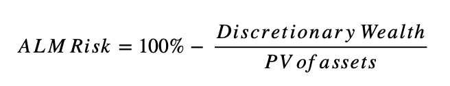
Lower ALM Risk means you have plenty of discretionary wealth, i.e. a riskless portfolio easily meets your goals with certainty, and you hence have more room to express risky preferences in portfolios while still meeting your goals with certainty.  Higher ALM Risk means you are just barely going to meet your goals with a low-risk portfolio, and to ensure meeting those goals, one shouldn’t be afforded the luxury of expressing their risk preferences.  And it’s critical to note that ALM above 100% means a risk-free portfolio cannot achieve the specified goals, and the goals need to be modified to the point that ALM gets down to 100% or lower, via tough conversations like saving more, working longer, lowering spending in retirement, etc.

Incorporating ALM into Asset Allocation

To account for the goals defined by the assets and liabilities within the ALM Risk calculation when building client portfolios, we will now moderate the client’s risk preferences toward less risky portfolios as ALM Risk goes up, bringing clients to a risk-free portfolio as ALM Risk nears 100%, and moderating portfolio risk preferences less and less as ALM Risk goes down, until we don’t moderate at all when ALM Risk is 0.  This process is outlined in Table 1.  

Table 1 Moderating Risk Preferences to Achieve Goals

	Measured	Moderated
Risk Aversion	ϒ	Max (ϒ, 1.5+10.5*SLR)
Loss Aversion	λ	Min (λ, 3-2*SLR)
Reflection	ϕ	Min (ϕ, 1.5+10.5*SLR)

Again, this system rests on two strong premises: that financial goals that are inflexible should be treated with high probabilities of success and that portfolio risk levels should never be pushed past client preferences.  Starting with a straight-line, deterministic Monte Carlo result, we can slowly open up our client portfolios to their desired risk levels as ALM Risk drops from 100%.  

Parting Words

Accounting for portfolio goals should be a priority for fiduciaries, and we have argued that as long as you don’t push clients past their risk comfort levels, portfolio goals should be the first feature we account for, even more important than risk preferences.  We have shown that if one systematically tilts client portfolios from full expression of risk preference to risk-free portfolios as goals become more and more lofty, we can build portfolios focused on goals while respecting client risk tolerances.

The 3-D Utility Function

To build portfolios that are truly tailored to an individual’s risk profile, one must account for all three of the primary risk preferences expressed by humans:  risk aversion, loss aversion, and reflection.  In what follows we begin by reviewing how portfolios can be constructed from a utility function.  We then show how one can easily extend the classic mean-variance approach, solely focused on risk aversion, to a more realistic 3-D risk preference paradigm, which additionally incorporates loss aversion and reflection.

What is Expected Utility Optimization?

To find the ideal investment portfolio for a human being we must calculate the expected utility (EU) for every possible portfolio, i.e. combination of assets, and choose the portfolio with the highest EU.  In this framework, the EU for a single portfolio is defined as:

Equation 1 Portfolio Expected Utility

where we sum over all O possible portfolio utility outcomes Uporti over the next time period (we use one-month forward-looking steps here), each with probability pⁱ, and where an outcome is defined as the joint return outcome of all assets during the next month.

Let’s for the moment assume our client’s utility function is the power utility function:

Equation 2 Power Utility

where W is the one-month wealth change 1 + r_p, r_p is the one-month period portfolio return, and γ is risk aversion (parameterized between 1.5 and 12).

In Table 1 we do a simple brute force EU optimization for two different portfolios and three possible outcomes, to keep things simple.  We first calculate the utility of each portfolio in each outcome, and then find the average across all outcomes for each portfolio.  The expected utility of Portfolio 1 is greater than the expected utility of Portfolio 2, making Portfolio 1 the optimal solution.  Of course, in practice, we would deploy an optimizer so we could choose amongst all possible portfolios and incorporate a much larger number of potential outcomes.  

Table Brute Force EU Optimization; Assumes γ = 3.

Portfolio 1: Stock 75%, Bonds 25%

Portfolio 2: Stock 60%, Bonds 40%

Now it turns out that a simpler problem to solve, mean-variance optimization, is a terrific approximation to the problem we just solved, which is precisely how Modern Portfolio Theory and its return vs. volatility paradigm became so popular.  But this function has no information on loss aversion or reflection, key risk preference dimensions discovered in the 1970s.  This function also has no information on skew or higher moments, a deficit increasingly of relevance in today’s markets.

What is a 3-D Utility Function?

Kahneman and Tversky introduced us to Prospect Theory in 1979, a key advancement in our understanding of decision making under uncertainty.  This theory of human behavior introduced two new features of decision making to the classical theory encapsulated by the Power utility function.

We could approximate Equation 2 very closely by:

Equation 3 Power Utility Approximated by a Quadratic Utility

When we then go to find the EU of the portfolio with this utility function we find the classic mean-variance result:

Equation 4 Mean-Variance Approximation to EU when Using Power Utility

1. Loss Aversion – the pain of losses is disproportionately greater than the pleasure of gains.  The more loss aversion one has, the more unwilling they will be to play a game with very favorable terms if there is a possibility of losing even small amounts.  
2. Reflection – investors are risk averse in the gain domain but risk-seeking in the loss domain.  We “hope to avoid losses” (risk-seeking in the loss domain) while being “afraid of missing gains” (risk-averse in the gain domain).

Incorporation of these two new dimensions of risk preferences in client portfolios is as simple as just inputting the refined utility function into Equation 1.  And now a mean-variance approximation is no longer a good approximation for client utility, while simultaneously addressing the lack of higher moments that are much more present in today’s markets.  The formula for this updated utility function gets a bit crazy, so its best to just to show how each preference updates the power utility function.

Figure 1 Moving from a 1D to 3D Utility Function

Figure 1 highlights how loss aversion generally pushes investors into portfolios with less volatility and less negative skew, since losses are so despised.  We also see how reflection can lead to riskier portfolios, as the utility functions is curved upward in the loss regime, and will generally push portfolios in the opposite “risk” direction as loss aversion.

Parting Words 

We now know, after decades of behavioral research advances, that human beings are not defined by a single risk parameter.  By extending risk profiling to the two additional risk preference dimensions of loss aversion and reflection, portfolios have a much better shot at more accurately representing a client’s risk profile, while simultaneously accounting for higher order moments that are now omnipresent in today’s markets.